Sparklines is new in Microsoft Excel 2010, a sparkline is a tiny chart in a worksheet cell that provides a visual representation of data. This tutorial helps you how to create Sparklines use Excel Functions. Note: this tutorial works well in excel 2003, 2007, 2010, 2013.
What is Sparklines?
A sparkline is a very small line chart, typically drawn without axes or coordinates. It presents the general shape of the variation (typically over time) in some measurement, such as temperature or stock market price, in a simple and highly condensed way. Sparklines are small enough to be embedded in text, or several sparklines may be grouped together as elements of a small multiple.
from WikiPedia
How To Create Sparklines Use Excel Functions
REPT() function repeats a piece of text a specified number of times. Use REPT to fill a cell with a number of instances of a text string. so, we can use REPT Function to create Sparklines.
REPT Function Syntax
REPT(text,number_times)
Text is the text you want to repeat.
Number_times is a positive number specifying the number of times to repeat text.
Sparkline Example 1
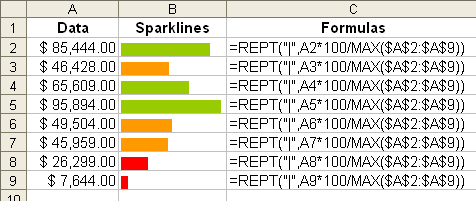
- Select A2, and input below formulas:
=INT(RAND()*10000) - Select B2, and input below formulas:
=REPT("|",A2*100/MAX($A$2:$A$9)) - Set B2 Font = Playbill, and Font Color = Lime
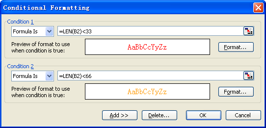
- select B2, click Menu Bar: Format, then click Conditional Formatting
Codition 1, select Formula Is, input the formula:=LEN(B2)<33, click Format, set Font Color = Red
Codition 2, select Formula Is, input the formula:=LEN(B2)<66, click Format, set Font Color = Light Orange
Sparkline Example 2
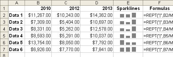
- Select B2:D2, and input below formulas:
=INT(RAND()*10000)+5000press Ctrl+Enter to end input.
- Select E2, and input below formulas:
=REPT("|",B2/MAX($B2:$D2)*15)&CHAR(10)&REPT("|",C2/MAX($B2:$D2)*15)&CHAR(10)&REPT("|",D2/MAX($B2:$D2)*15) - Select E2, press Ctrl+1, click Alignment, set
Horizontal: Center
Vertical: Bottom
Choose Wrap text
Orientation = 90 Degrees
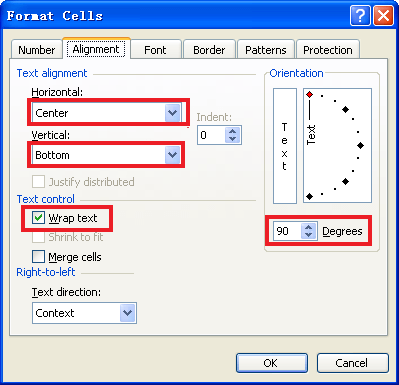
- Set E2 Font = Playbill, and Font Color = Gray-50%
Sparkline Example 3
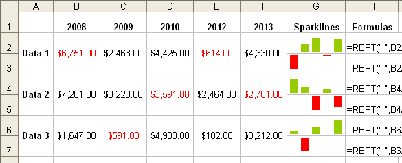
- Select A2, and input below formulas:
=INT(RAND()*10000)press Ctrl+Enter to end input.
- Select G2, and input below formulas:
=REPT("|",B2/MAX($B2:$F2)*20*(B2>=0))&CHAR(10)&REPT("|",C2/MAX($B2:$F2)*20*(C2>=0))&CHAR(10)&REPT("|",D2/MAX($B2:$F2)*20*(D2>=0))&CHAR(10)&REPT("|",E2/MAX($B2:$F2)*20*(E2>=0))&CHAR(10)&REPT("|",F2/MAX($B2:$F2)*20*(F2>=0)) - Set G2 Font = Playbill, and Font Color = Lime
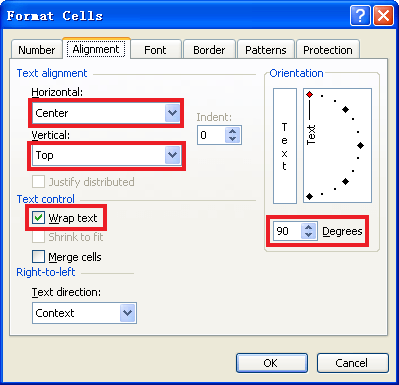
- Select G2, press Ctrl+1, click Alignment, set
Horizontal: Center
Vertical: Bottom
Choose Wrap text
set Orientation = 90 Degrees
- Select G3, and input below formulas:
=REPT("|",B2/MIN($B2:$F2)*20*(B2<0))&CHAR(10)&REPT("|",C2/MIN($B2:$F2)*20*(C2<0))&CHAR(10)&REPT("|",D2/MIN($B2:$F2)*20*(D2<0))&CHAR(10)&REPT("|",E2/MIN($B2:$F2)*20*(E2<0))&CHAR(10)&REPT("|",F2/MIN($B2:$F2)*20*(F2<0)) - Select G3, press Ctrl+1, click Alignment, set
Horizontal: Center
Vertical: Top
Choose Wrap text
set Orientation = 90 Degrees
- Set G3 Font = Playbill, and Font Color = Red
Thanks for the great post. Works a treat although you need to use char(13) for the formula to render correctly.
A generic way to determine the operating system is via this function
=IF(INFO("system")="mac",CHAR(13),CHAR(10))
thanks for the tutorial! This was exactly what i was looking for!!
Hello,
While I was going through this tutorial, I just thought of sharing an experience of mine. I recently came across this site,jolicharts. For data visualization and creating charts derived directly from excel sheets.
It was good for me as day to day charting and data presentation was taking way too much of my time..
I hope this info also might help few more of us.
Well no harm in trying it for free..